Finding Particles Within a Shape¶

We have 4 goals for this tutorial:

Create some particle position data
Create a ParticleCubes object
Find all the particles in a square
Find all the particles within a circle

We'll assume you already are somewhat familiar with numpy and matplotlib.

We'll keep everything in 2D to make plotting easier, but all of these steps can be done in 1D & 3D as well¹.

Code cells and the terminal

The code cells in this tutorial are intended for use in/copying to python notebook (.ipynb) or ipython inputs and so have many plot commands that would be unnecessary or require plt.show() constantly for someone experimenting from e.g. the terminal. If you are such a user, we'll denote a cell with plot commands that you may want to use like so:

plt.plot(...) # (1)!

Run plt.show() after these commands

And any cell that does not have such an annotation you can ignore all lines starting with plt.

Install and Import Dependencies¶

Since we'll be using matplotlib for visualization, we'll want to include the viz optional dependencies:

pippixi

$ pip install "packingcubes[viz]

$ pixi add packingcubes[viz] --pypi

Now import the modules we need

import numpy as np
import matplotlib.pyplot as plt

import packingcubes

Create positions data¶

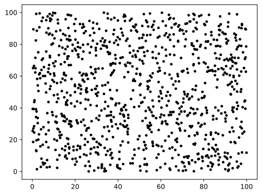
We'll start by generating some random data. We'll make 1000 particles with \(x\) and \(y\) coordinates ranging from 0 to 100.

xy = np.random.uniform(size=(1000,2)) * 100

plt.plot(xy[:,0], xy[:,1] , "k.")
plt.savefig("PWS_figs/fig_1.svg", bbox_inches="tight") # (1)!

You can ignore lines, they're temporary fixes for issues rendering images in the docs

Figure 1: Random arrangement of points

ParticleCubes are designed to work with 3D data, so we'll need to pad our 2D data with zeros to make it 3D.

positions = np.zeros_like(xy, shape=(len(xy),3))
positions[:, :2] = xy

1D/2D data and OpTrees

OpTrees will do this padding for you at the cost of being a little more opaque, and only working with position data. Note that packingcubes will be 4x/2x slower creating the tree than a dedicated binary- or quad-tree would be. Search should still be comparable, however.

Create a ParticleCubes object¶

We don't need anything fancy, so creating a ParticleCubes is pretty simple:

cubes = packingcubes.Cubes(positions, particle_threshold=10) # (1)!
cubes

You normally wouldn't specify the particle_threshold. It's only done here to create multiple data chunks for the plots.

Find all particles in a square¶

Define our square¶

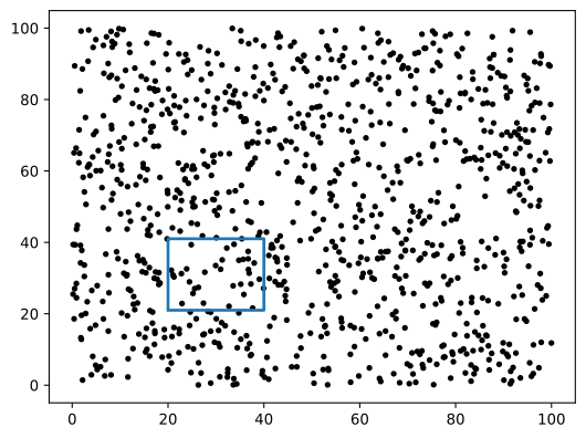
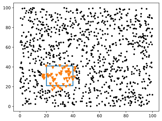
We'll look at the square whose bottom-left corner is \((20, 21)\) and that has a side-length of 10.

plt.plot(xy[:,0], xy[:,1] , "k.")
bx = 20
by = 21
side = 20
plt.plot(bx + np.array([0, side, side, 0, 0]), by + np.array([0, 0, side, side, 0]), lw=2)
plt.savefig("PWS_figs/fig_2.svg", bbox_inches="tight")

Figure 2: Random arrangement of points with a box

To search in a box, we set the corner position and then the dimensions of the box as a single array in the form [x, y, z, dx, dy, dz].

Unfortunately, ParticleCubes do not currently support 1D or 2D search shapes. Luckily, making our square 3D is easy, just set the \(z\) position to 0:

box = [bx, by, 0, side, side, side] # (1)!

Having a 3D search volume with 2D data is fine, packingcubes will effectively just ignore the third dimension. The only caveat is you need to ensure the box actually has a volume. Setting dz=0 would raise an error.

Actually do the search¶

We'll do the search in 3 different ways, corresponding to different use-cases:

Chunk indices¶

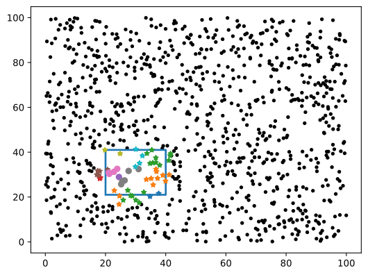
index_array = cubes.get_particle_indices_in_box(box)

Index array is an array of data chunk indices, where each row represents a data chunk in the form [start, stop, partial]. partial just specifies if the entire chunk is contained (0) or if it's only partially contained (1).

plt.plot(xy[:,0], xy[:,1] , "k.") # (1)!
plt.plot(bx + np.array([0, side, side, 0, 0]), by + np.array([0, 0, side, side, 0]), lw=2)

for start, stop, partial in index_array:
    # plot each chunk of data
    chunk = positions[start:stop, :2]
    plt.plot(chunk[:,0], chunk[:, 1], "*" if partial else "o") # (2)!
plt.savefig("PWS_figs/fig_3.svg", bbox_inches="tight")

Run plt.show() after these commands
Using different markers for the different partial values is purely for visual effect, there's no difference between the chunks.

Figure 3: Displaying the particles in the different chunks

Best for high performance

This method will give results in the shortest possible time (since there's no sorting or strict containment checks) and is intended for loading data from files. It also does not require any information from the dataset, everything needed is already included in the cubes structure, and so uses the least amount of memory.

Index lists¶

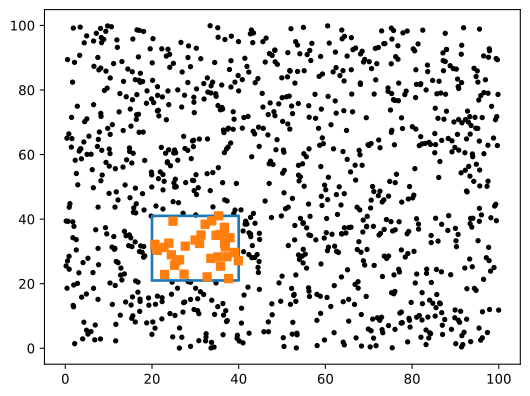
index_list = cubes.get_particle_index_list_in_box(box, strict=True)

Array of indices into the positions array. With this method, you can specify whether particles must strictly be inside the box (shown), or if you want the indices in the original unsorted data (use_data_indices=False, not shown).

plt.plot(xy[:,0], xy[:,1] , "k.") # (1)!
plt.plot(bx + np.array([0, side, side, 0, 0]), by + np.array([0, 0, side, side, 0]), lw=2)

plt.plot(positions[index_list,0], positions[index_list, 1], "s")
plt.savefig("PWS_figs/fig_4.svg", bbox_inches="tight")

Run plt.show() after these commands

Figure 4: Displaying strict particle search

Best for parity with SciPy's KDTree

These results will be the most similar to SciPy's KDTree output, but note that it's almost always more performant to use index slices, like in chunk indices, than actual indexes, especially if you expect many of them. This method requires access to the dataset (usually already included).

Search Objects¶

(name WIP, suggestions welcome!)

search_positions = cubes.Box(box, strict=False).positions # (1)!

You can get the same strictness check as with index lists by setting strict=True

This will return the actual positions of the particles in the box. Note that you can't get the direct particle indices in this fashion, but you can obtain other fields besides positions via this method². See Temperature vs Radii of a Halo using Search Objects for an example.

plt.plot(xy[:,0], xy[:,1] , "k.") # (1)!
plt.plot(bx + np.array([0, side, side, 0, 0]), by + np.array([0, 0, side, side, 0]), lw=2)

plt.plot(search_positions[:,0], search_positions[:, 1], "v")
plt.savefig("PWS_figs/fig_5.svg", bbox_inches="tight")

Run plt.show() after these commands

Figure 5: Displaying strict particle search

Best for looking at multiple fields of the particles

This method will give you a subdataset with all the extra fields you request. You can also request strict containment checks. This method requires access to the positions and any extra fields defined, and can use a lot more memory.

Find all particles in a circle¶

Define the circle¶

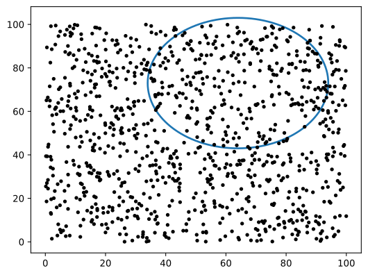
We'll look at the circle centered at \((64, 73)\) with radius \(30\).

Note that this circle extends outside our data bounds!

We'll need to do the same z=0 trick when converting to a 3D sphere.

center = [64, 73, 0]
radius = 30

plt.plot(xy[:,0], xy[:,1] , "k.")
circle = plt.Circle(
    center[:2], radius, color='tab:blue', 
    lw=2, clip_on=False, fill=False
)
plt.gca().add_patch(circle)
plt.savefig("PWS_figs/fig_6.svg", bbox_inches="tight")

Figure 6: Random arrangement of points with a circle

Actually do the search¶

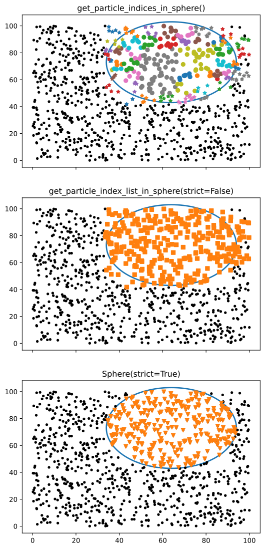
This works pretty much identically to the square (box), so we'll do all three types at once:

index_array = cubes.get_particle_indices_in_sphere(center=center, radius=radius)
index_list = cubes.get_particle_index_list_in_sphere(
    center=center, radius=radius, strict=False
) # (1)!
search_positions = cubes.Sphere(
    center=center, radius=radius, strict=True
).positions

We've swapped the strictness tests for demonstration purposes

fig, axs = plt.subplots(3,1, sharey=True, sharex=True) # (1)!
fig.set_figheight(14)
for ax in axs:
    ax.plot(xy[:,0], xy[:,1] , "k.")
    circle = plt.Circle(
        center[:2], radius, color='tab:blue',
        lw=2, clip_on=False, fill=False
    )
    ax.add_patch(circle)

# plot index_array
for start, stop, partial in index_array:
    # plot each chunk of data
    chunk = positions[start:stop, :2]
    axs[0].plot(chunk[:,0], chunk[:, 1], "*" if partial else "o") # (2)!
axs[0].set_title("get_particle_indices_in_sphere()")

# plot index_list
axs[1].plot(
    positions[index_list,0], positions[index_list, 1],
    "s",color="tab:orange"
)
axs[1].set_title("get_particle_index_list_in_sphere(strict=False)")

# plot Sphere
axs[2].plot(
    search_positions[:,0], search_positions[:, 1],
    "v", color="tab:orange"
)
axs[2].set_title("Sphere(strict=True)")

plt.savefig("PWS_figs/fig_7.svg", bbox_inches="tight")

Run plt.show() after these commands
Just like above, using different markers for the different partial values is purely for visual effect, there's no difference between the chunks.

Figure 7: Particles in sphere, 3 ways

Fragile Data!

You may notice that the order of the data in positions has changed (occurred when we made cubes). This is by design! But it also means if you modify positions you will break the linkage between search results and the data. For more on this, see Working with Datasets for more robust ways to interact with data.

Summary¶

Below is a table of the different methods used here as well as some notes:

Desired result...	in a Box.	in a Sphere.	Notes
particle index chunks as fast as possible	`get_particle_indices_in_box(box)`	`get_particle_indices_in_sphere(center, radius)`	Minimal memory use, fastest performance, need to process index chunks
actual particle indices	`get_particle_index_list_in_box(box)`	`get_particle_index_list_in_sphere(center, radius)`	Closest to SciPy's KDTree, can do strict containment tests. How often do you actually need the particle indices?
Multiple data fields in a region	`Box(box)`	`Sphere(center, radius)`	Returns a subdataset, with fields available as `.field_name`. Requires some additional setup²³. Grabs every field specified, potentially taking more time, memory, but is reusable.

The packingcubes portions are actually much simpler in 3D, as will become obvious shortly, but the plotting becomes a lot harder. ↩
See Sorting Additional Fields and All-in-One for how to specify them. ↩↩
See Temperature vs Radii of a Halo using Search Objects for an example of the additional setup. ↩